Read Mapping Statistics

The sample is sequenced as non-stranded RNA-seq

#==================================================
#All numbers are READ count
#==================================================

Total records:                          187092760

QC failed:                              0
Optical/PCR duplicate:                  0
Non primary hits                        57239324
Unmapped reads:                         0
mapq < mapq_cut (non-unique):           35882554

mapq >= mapq_cut (unique):              93970882
Read-1:                                 46985441
Read-2:                                 46985441
Reads map to '+':                       46985441
Reads map to '-':                       46985441
Non-splice reads:                       82606072
Splice reads:                           11364810
Reads mapped in proper pairs:           93970882
Proper-paired reads map to different chrom:0

read_distribution

Provided a BAM/SAM file and reference gene model, this module will calculate how mapped reads were distributed over genome feature (like CDS exon, 5’UTR exon, 3’ UTR exon, Intron, Intergenic regions). When genome features are overlapped (e.g. a region could be annotated as both exon and intron by two different transcripts) , they are prioritize as: CDS exons > UTR exons > Introns > Intergenic regions, for example, if a read was mapped to both CDS exon and intron, it will be assigned to CDS exons.

• “Total Reads”: This does NOT include those QC fail,duplicate and non-primary hit reads
• “Total Tags”: reads spliced once will be counted as 2 tags, reads spliced twice will be counted as 3 tags, etc. And because of this, “Total Tags” >= “Total Reads”
• “Total Assigned Tags”: number of tags that can be unambiguously assigned the 10 groups (see below table).
• Tags assigned to “TSS_up_1kb” were also assigned to “TSS_up_5kb” and “TSS_up_10kb”, tags assigned to “TSS_up_5kb” were also assigned to “TSS_up_10kb”. Therefore, “Total Assigned Tags” = CDS_Exons + 5’UTR_Exons + 3’UTR_Exons + Introns + TSS_up_10kb + TES_down_10kb.
• When assign tags to genome features, each tag is represented by its middle point.

RSeQC cannot assign those reads that:

• hit to intergenic regions that beyond region starting from TSS upstream 10Kb to TES downstream 10Kb.
• hit to regions covered by both 5’UTR and 3’ UTR. This is possible when two head-to-tail transcripts are overlapped in UTR regions.
• hit to regions covered by both TSS upstream 10Kb and TES downstream 10Kb.

processing /home/statonse/db/Ha412v1r1_genes_v1.0.bed ... Done

Total Reads                   129853436
Total Tags                    144000059
Total Assigned Tags           99967932
=====================================================================
Group               Total_bases         Tag_count           Tags/Kb             
CDS_Exons           50673964            74716289            1474.45           
5'UTR_Exons         0                   0                   0.00              
3'UTR_Exons         0                   0                   0.00              
Introns             83648462            3600196             43.04             
TSS_up_1kb          42018537            1185417             28.21             
TSS_up_5kb          195923394           6888549             35.16             
TSS_up_10kb         370551414           9728871             26.26             
TES_down_1kb        40257870            4831071             120.00            
TES_down_5kb        183624376           8819561             48.03             
TES_down_10kb       353055864           11922576            33.77             
=====================================================================

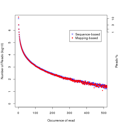
read_duplication

Two strategies were used to determine reads duplication rate: * Sequence based: reads with exactly the same sequence content are regarded as duplicated reads. * Mapping based: reads mapped to the same genomic location are regarded as duplicated reads. For splice reads, reads mapped to the same starting position and splice the same way are regarded as duplicated reads.

read_GC

Distribution of reads vs. percentages of GC content.

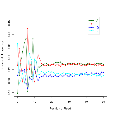
read_NVC

This module is used to check the nucleotide composition bias. In ideal condition (genome is random and RNA-seq reads is randomly sampled from genome), we expect A%=C%=G%=T%=25% at each position of reads. It is perfectly normal to observe both a slight GC bias and a distinctly non-random base composition over the first 12 bases of the data. This is observed when looking, for instance, at the IVC (intensity versus cycle number) plots which are part of the output of the Pipeline. In genomic DNA sequencing, the base composition is usually quite uniform across all bases; but in mRNA-Seq, the base composition is noticeably uneven across the first 10 to 12 bases. Illumina believes this effect is caused by the "not so random" nature of the random priming process used in the protocol. This may explain why there is a slight overall G/C bias in the starting positions of each read. The first 12 bases probably represent the sites that were being primed by the hexamers used in the random priming process. The first twelve bases in the random priming full-length cDNA sequencing protocol (mRNA-seq) always have IVC plots that look like what has been described. This is because the random priming is not truly random and the first twelve bases (the length of two hexamers) are biased towards sequences that prime more efficiently.This is entirely normal and expected. This bias could be easily examined by NVC (Nucleotide versus cycle) plot. NVC plot is generated by overlaying all reads together, then calculating nucleotide composition for each position of read (or each sequencing cycle).

NOTE: this program expect a fixed read length

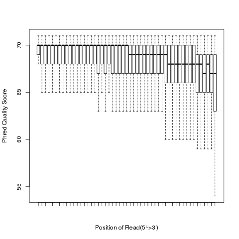
read_quality

According to SAM specification, if Q is the character to represent “base calling quality” in SAM file, then Phred Quality Score = ord(Q) - 33. Here ord() is python function that returns an integer representing the Unicode code point of the character when the argument is a unicode object, for example, ord(‘a’) returns 97. Phred quality score is widely used to measure “reliability” of base-calling, for example, phred quality score of 20 means there is 1/100 chance that the base-calling is wrong, phred quality score of 30 means there is 1/1000 chance that the base-calling is wrong. In general: Phred quality score = -10xlog(10)P, here P is probability that base-calling is wrong.

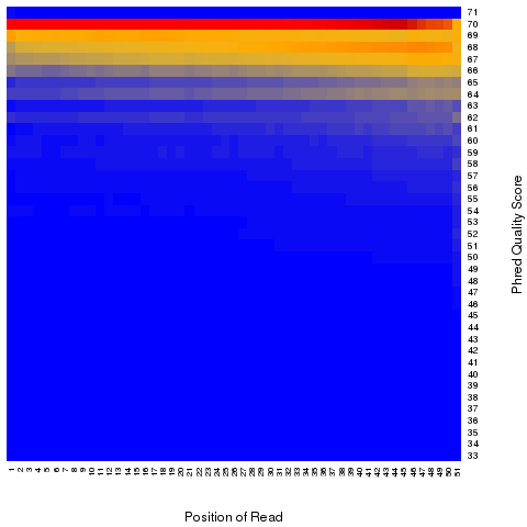
Heatmap: use different color to represent nucleotide density (“blue”=low density,”orange”=median density,”red”=high density”)

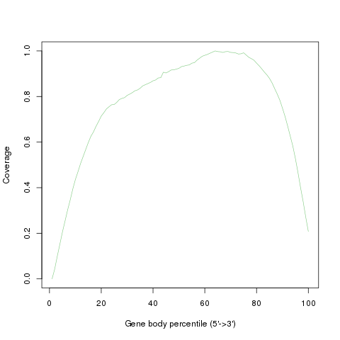
geneBody_coverage

Read coverage over gene body. This module is used to check if reads coverage is uniform and if there is any 5’/3’ bias. This module scales all transcripts to 100 nt and calculates the number of reads covering each nucleotide position. Finally, it generates a plot illustrating the coverage profile along the gene body.

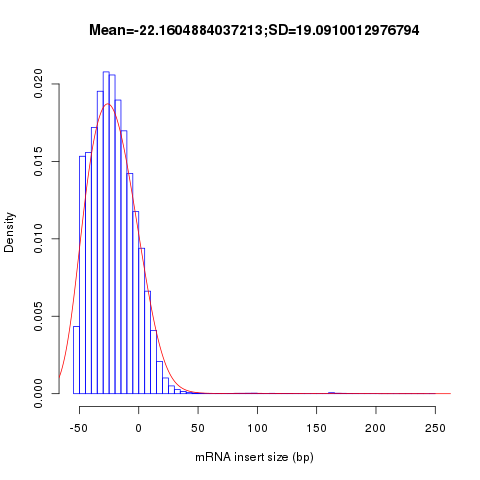
inner_distance

This module is used to calculate the inner distance (or insert size) between two paired RNA reads. The distance is the mRNA length between two paired fragments. We first determine the genomic (DNA) size between two paired reads: D_size = read2_start - read1_end, then

• if two paired reads map to the same exon: inner distance = D_size
• if two paired reads map to different exons:inner distance = D_size - intron_size
• if two paired reads map non-exonic region (such as intron and intergenic region): inner distance = D_size
• The inner_distance might be a negative value if two fragments were overlapped.

NOTE: Not all read pairs were used to estimate the inner distance distribution. Those low quality, PCR duplication, multiple mapped reads were skipped.

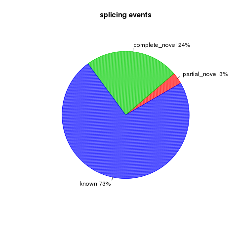
junction_annotation

This program will compare detected splice junctions to reference gene model. splicing annotation is performed in two levels: splice event level and splice junction level.

• splice event: An RNA read, especially long read, can be spliced 2 or more times, each time is called a splicing event; In this sense, 100 spliced reads can produce >= 100 splicing events.
• splice junction: multiple splicing events spanning the same intron can be consolidated into one splicing junction.

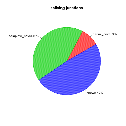
All detected junctions can be grouped to 3 exclusive categories:

1. Annotated: The junction is part of the gene model. Both splice sites, 5’ splice site (5’SS) and 3’splice site (3’SS) can be annotated by reference gene model.
2. complete_novel: Complete new junction. Neither of the two splice sites cannot be annotated by gene model
3. partial_novel: One of the splice site (5’SS or 3’SS) is new, while the other splice site is annotated (known)

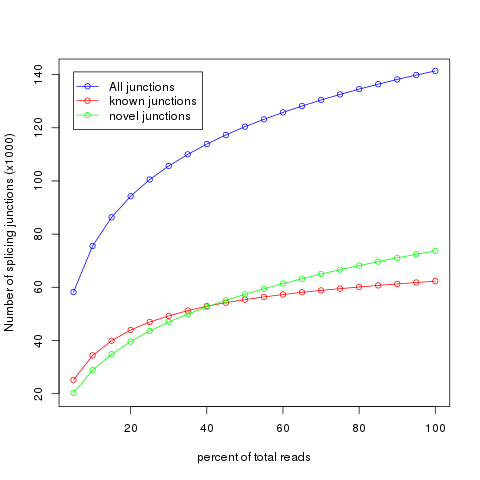
junction_saturation

It’s very important to check if current sequencing depth is deep enough to perform alternative splicing analyses. For a well annotated organism, the number of expressed genes in particular tissue is almost fixed so the number of splice junctions is also fixed. The fixed splice junctions can be predetermined from reference gene model. All (annotated) splice junctions should be rediscovered from a saturated RNA-seq data, otherwise, downstream alternative splicing analysis is problematic because low abundance splice junctions are missing. This module checks for saturation by resampling 5%, 10%, 15%, ..., 95% of total alignments from BAM or SAM file, and then detects splice junctions from each subset and compares them to reference gene model.